Getting Started with R and RStudio

# Getting Started with R and RStudio
### Jessica Minnier, PhD & Meike Niederhausen, PhD <a href="https://www.ohsu.edu/xd/research/centers-institutes/octri/education-training/octri-research-forum.cfm">OCTRI Biostatistics, Epidemiology, Research & Design (BERD) Workshop</a> 
### 2019/09/24 & 2020/02/19 slides: <a href="http://bit.ly/berd_intro_r">bit.ly/berd_intro_r</a> pdf: <a href="http://bit.ly/berd_intro_r_pdf">bit.ly/berd_intro_r_pdf</a>

---

---

# 1. Open slides: [bit.ly/berd_intro_r](http://bit.ly/berd_intro_r)

## 2. Install R

- Windows: 
    - Download from https://cran.rstudio.com/bin/windows/base/
- Mac OS X: 
    - Download the latest .pkg file (currently R-3.6.2.pkg) from https://cran.rstudio.com/bin/macosx/

## 3. Install RStudio Desktop Open Source License

- Select download file corresponding to your operating system  from https://www.rstudio.com/products/rstudio/download/#download

## 4. Download folder of data (unzip completely)

- Go to [bit.ly/intro_rproj](http://bit.ly/intro_rproj) and **unzip** folder
- Open (double click on) `berd_intro_project.Rproj` file.

---

# Questions

- Who has used R?
- What other statistical software have you used?
- Has anyone used other programming languages (C, java, python, etc)?
- Why do you want to learn R?

---

# Learning Objectives

- Basic operations in R/RStudio
- Understand data structures
- Be able to load in data
- Basic operations on data
- Be able to make a plot
- Know how to get help

---
class: center, inverse, middle

# Introduction

Rrrrrr?

---

# What is R?

.pull-left-60[
- A programming language
- Focus on statistical modeling and data analysis
    + import data, manipulate data, run statistics, make plots
- Useful for "Data Science"
- Great visualizations
- Also useful for most anything else you'd want to tell a computer to do
- Interfaces with other languages i.e. python, C++, bash

]

For the history and details: [Wikipedia](https://bit.ly/1efFmaY)

- an interpreted language (run it through a command line)
- procedural programming with functions
- Why "R"?? Scheme (?) inspired S (invented at Bell Labs in 1976) which inspired R (**free and open source!** in 1992)

---

# What is RStudio?

.pull-left[
R is a programming language]
.pull-right[
RStudio is an integrated development environment (IDE) = an interface to use R (with perks!)
]

<center><img src="img/01_md_rstudio.png" width="78%" height="78%"><a href="https://moderndive.com/1-getting-started.html#r-rstudio"> Modern Dive</a></center>

---

# Start RStudio

## Double click on the `berd_intro_project.Rproj` file.

<center><img src="img/01_md_r.png" width="78%" height="78%"><a href="https://moderndive.com/1-getting-started.html#using-r-via-rstudio"> Modern Dive</a></center>
---

---

# Rstudio demo

---

# R Projects (why .Rproj file?) & Good Practices

__Use projects to keep everything together__ ([read this](https://r4ds.had.co.nz/workflow-projects.html))
- Create an RStudio project for each data analysis project, for each homework assignment, etc.
- A project is associated with a directory folder
    + Keep data files there
    + Keep scripts there; edit them, run them in bits or as a whole
    + Save your outputs (plots and cleaned data) there
- Only use relative paths, never absolute paths
    + relative (good): `read.csv("data/mydata.csv")`
    + absolute (bad): `read.csv("/home/yourname/Documents/stuff/mydata.csv")`
    
__Advantages of using projects__
- standardizes file paths
- keep everything together
- a whole folder can be easily shared and run on another computer
- when you open the project everything is as you left it

---

# Let's code!

---

# Coding in the console 
 
.pull-left[
__Typing and execting code in the console __
* Type code in the console
* Press __return__ to execute the code
* Output shown below

_Coding in the console is not advisable for most situations!_
* We only recommend this for short pieces of code that you don't need to save
* We will be using scripts (`.R` files) to run and save code (in a few slides)

```r
> 7
```

```
[1] 7
```

]

```r
> 3 + 5
```

```
[1] 8
```

```r
> "hello"
```

```
[1] "hello"
```

```r
> # this is a comment, nothing happens
> # 5 - 8
> 
> # separate multiple commands with ;
> 3 + 5; 4 + 8
```

```
[1] 8
```

```
[1] 12
```
]

---

# We can do math

```r
> 10^2
```

```
[1] 100
```

```r
> 3 ^ 7
```

```
[1] 2187
```

```r
> 6/9
```

```
[1] 0.6666667
```

```r
> 9-43
```

```
[1] -34
```
]

.pull-right[
R follows the rules for order of operations and ignores spaces between numbers (or objects)

```r
> 4^3-2* 7+9 /2
```

```
[1] 54.5
```

The equation above is computed as `$$4^3 − (2 \cdot 7) + \frac{9}{2}$$` 
]

---

# Logarithms and exponentials

Logarithms: `log()` is base `$e$`

```r
> log(10)
```

```
[1] 2.302585
```

```r
> log10(10)
```

```
[1] 1
```

]

```r
> exp(1)
```

```
[1] 2.718282
```

```r
> exp(0)
```

```
[1] 1
```
]

Check that `log()` is base `$e$`

```r
> log(exp(1))
```

```
[1] 1
```

---

# Using functions

* `log()` is an example of a function
* functions have "arguments"
* `?log` in console will show help for `log()`

```r
> mean(1:4)
```

```
[1] 2.5
```

```r
> seq(1,12,3)
```

```
[1]  1  4  7 10
```
]
.pull-right[
Arguments read by name:

```r
> mean(x = 1:4)
```

```
[1] 2.5
```

```r
> seq(from = 1, to = 12, by = 3)
```

```
[1]  1  4  7 10
```
]

---

# Variables

Data, information, everything is stored as a variable
.pull-left[
* Can assign a variable using either `=` or `<-`
 - Using `<-` is preferable
 - type name of variable to print

Assigning just one value:

```r
> x = 5
> x
```

```
[1] 5
```

```r
> x <- 5
> x
```

```
[1] 5
```
]

```r
> a <- 3:10
> a
```

```
[1]  3  4  5  6  7  8  9 10
```

* __Concatenate__ a string of numbers

```r
> b <- c(5, 12, 2, 100, 8)
> b
```

```
[1]   5  12   2 100   8
```
]

---

# We can do math with variables

```r
> x <- 5
> x
```

```
[1] 5
```

```r
> x + 3
```

```
[1] 8
```

```r
> y <- x^2
> y
```

```
[1] 25
```
]

```r
> a <- 3:6
> a
```

```
[1] 3 4 5 6
```

```r
> a+2; a*3
```

```
[1] 5 6 7 8
```

```
[1]  9 12 15 18
```

```r
> a*a
```

```
[1]  9 16 25 36
```
]

---

# Variable can include text (characters)

```r
> hi <- "hello"
> hi
```

```
[1] "hello"
```

```r
> greetings <- c("Guten Tag", "Hola", hi)
> greetings
```

```
[1] "Guten Tag" "Hola"      "hello"    
```

---

# Missing values

Missing values are denoted as `NA` and are handled differently depending on the operation. There are special functions for `NA` (i.e. `is.na()`, `na.omit()`).
.pull-left[

```r
> x <- c(1, 2, NA, 5)
> is.na(x)
```

```
[1] FALSE FALSE  TRUE FALSE
```

```r
> mean(x)
```

```
[1] NA
```

```r
> mean(x, na.rm=TRUE)
```

```
[1] 2.666667
```
]
.pull-right[

```r
> x <- c("a", "a", NA, "b")
> table(x)
```

```
x
a b 
2 1 
```

```r
> table(x, useNA = "always")
```

```
x
 a b <NA> 
 2 1 1 
```

]

---

# Viewing list of defined variables

* `ls()` is the R command to see what objects have been defined. 
* This list includes all defined objects (including dataframes, functions, etc.)

```r
> ls()
```

```
[1] "a"         "b"         "greetings" "hi"        "x"         "y"        
```

* You can also look at the list in the Environment window: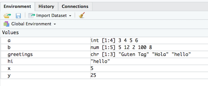

![](img/01_ls_screenshot.png)

---

# Removing defined variables

* The R command to delete an object is `rm()`.

```r
> ls()
```

```
[1] "a"         "b"         "greetings" "hi"        "x"         "y"        
```

```r
> rm("greetings", hi)  # Can run with or without quotes
> ls()
```

```
[1] "a" "b" "x" "y"
```

* Remove EVERYTHING - _Be careful!!_

```r
> rm(list=ls())
> ls()
```

```
character(0)
```
 
 * Can also remove everything using the _Clear Workspace_ option in the _Session_ menu.

---

# Common console errors (1/2)
 
__Incomplete commands__

.pull-left[
* When the console is waiting for a new command, the prompt line begins with `>`
  + If the console prompt is `+`, then a previous command is incomplete
  + You can finish typing the command in the console window
]
   
.pull-right[
Example:

```r
> 3 + (2*6
+ )
```

```
[1] 15
```
]

---

# Common console errors (2/2)

__Object is not found__

* This happens when text is entered for a non-existent variable (object)

Example:

```r
> hello
```

```
Error in eval(expr, envir, enclos): object 'hello' not found
```

* Can be due to missing quotes

```r
> install.packages(dplyr) # need install.packages("dplyr")
```

```
Error in install.packages(dplyr): object 'dplyr' not found
```
---

# R scripts (save your work!)

---

# Coding in a script (1/3)

* __Create a new script__ by 
    + selecting `File -> New File -> R Script`, 
    + *or* clicking on ![](img/01_Script_create.png) (the left most button at the top of the scripting window), and then selecting the first option `R Script`

* __Type code__ in the script
    - Type each R command on its own line
    - Use `#` to convert text to comments so that text doesn't accidentally get executed as an R command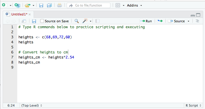

![](img/01_Scripting_practice1.png)
---

# Coding in a script (2/3)

* __Select code__ you want to execute, by 
    - placing the cursor in the line of code you want to execute, 
    - __*or*__ highlighting the code you want to execute

* __Execute code__ in the script, by
    - clicking on the ![](img/01_Script_Run.png) button in the top right corner of the scripting window, 
    - or typing one of the following key combinations to execute the code
          + __Windows__:  __ctrl + return__
          + __Mac__:  __command + return__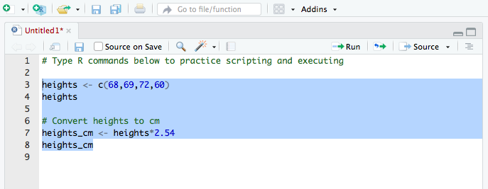

---

# Coding in a script (3/3)

* The screenshot below shows code in the scripting window (top left window)
* The executed highlighted code and its output appear in the console window (bottom left window)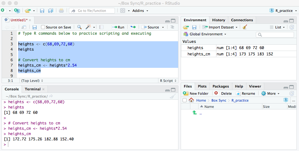

---

# Useful keyboard shortcuts

action | mac | windows/linux
---| ---| ---
run code in script | cmd + enter | ctrl + enter 
`<-`| option + - | alt + -
]
.pull-right-40[
Try typing (with shortcut) in a script and running

```r
y <- 5
y
```
Now, in the *console*, press the up arrow.
]

## Others: ([see full list](https://support.rstudio.com/hc/en-us/articles/200711853-Keyboard-Shortcuts))

action | mac | windows/linux
---| ---| ---
interrupt currently executing command | esc | esc
in console, go to previously run code | up/down | up/down
keyboard shortcut help | option + shift + k | alt + shift + k
---

# Saving a script

* __Save a script__ by 
    + selecting `File -> Save`, 
    + or clicking on ![](img/01_Script_Save.png) (towards the left above the scripting window)

* You will need to specify
    + a __filename__ to save the script as
        - ALWAYS use __.R__ as the filename extension for R scripts
    + the __folder__ to save the script in

---

# Practice time!

---

# Practice 1

1. Open a new R script and type code/answers for next tasks in it. Save as `Practice1.R`

1. Create a vector of all integers from 4 to 10, and save it as `a1`.

1. Create a vector of _even_ integers from 4 to 10, and save it as `a2`.

1. What is the sum of `a1` and `a2`?

1. What does the command `sum(a1)` do?

1. What does the command `length(a1)` do?

1. Use the `sum` and `length` commands to calculate the average of the values in `a1`.

1. Compute the sum of all integers from 1 to 100. Then compare your answer to the one you get using the formula for sum of the first `$n$` integers: `$n(n+1)/2$`.

1. Compute the sum of the squares of all integers from 1 to 100.

1. Take a break!

---

# Object types

---

# Data frames

.pull-left-60[
__Vectors__ vs. __data frames__: a data frame is a collection (or array or table) of vectors

```r
df <- data.frame(
 IDs=1:3, 
 gender=c("male", "female", "Male"), 
 age=c(28, 35.5, 31),
 trt = c("control", "1", "1"),
 Veteran = c(FALSE, TRUE, TRUE)
 )
df
```

```
##   IDs gender  age     trt Veteran
## 1   1   male 28.0 control   FALSE
## 2   2 female 35.5       1    TRUE
## 3   3   Male 31.0       1    TRUE
```

]
.pull-right-40[

* Allows different columns to be of different data types (i.e. numeric vs. text)
* Both numeric and text can be stored within a column (stored together as *text*).

* Vectors and data frames are examples of _**objects**_ in R. 
  + There are other types of R objects to store data, such as matrices, lists, and tibbles.
  + These will be discussed in future R workshops.
]

---

# Variable (column) types

type | description
---|---
integer | integer-valued numbers
numeric | numbers that are decimals
factor | categorical variables stored with levels (groups)
character | text, "strings"
logical | boolean (TRUE, FALSE)

* View the __structure__ of our data frame to see what the variable types are:

```r
str(df)
```

```
## 'data.frame':	3 obs. of  5 variables:
##  $ IDs    : int  1 2 3
##  $ gender : Factor w/ 3 levels "female","male",..: 2 1 3
##  $ age    : num  28 35.5 31
##  $ trt    : Factor w/ 2 levels "1","control": 2 1 1
##  $ Veteran: logi  FALSE TRUE TRUE
```

---

# Data frame cells, rows, or columns

.pull-left[
Show whole data frame

```r
df
```

```
##   IDs gender  age     trt Veteran
## 1   1   male 28.0 control   FALSE
## 2   2 female 35.5       1    TRUE
## 3   3   Male 31.0       1    TRUE
```

Specific cell value:

`DatSetName[row#, column#]`

```r
# Second row, Third column
df[2, 3]
```

```
## [1] 35.5
```
]

`DatSetName[, column#]`

```r
# Third column
df[, 3]
```

```
## [1] 28.0 35.5 31.0
```

Entire row: `DatSetName[row#, ]`

```r
# Second row
df[2,]
```

```
##   IDs gender  age trt Veteran
## 2   2 female 35.5   1    TRUE
```
]

---

# Getting the data into Rstudio

---

# Load a data set

* Read in csv file from file path with code (filepath relative to Rproj directory)

```r
mydata <- read.csv("data/yrbss_demo.csv")
```

* Or, open saved file using Import Dataset button in Environment window:  ![](img/01_Import_Dataset.png). 
  + If you use this option, then copy and paste the importing code to your script so that you have a record of from where and how you loaded the data set.

```r
View(mydata) 
# Can also view the data by clicking on its name in the Environment tab
```

---

# About the data

Data from the CDC's [Youth Risk Behavior Surveillance System (YRBSS) ](https://www.cdc.gov/healthyyouth/data/yrbs/index.htm)

- small subset (20 rows) of the full complex survey data
- national school-based survey conducted by CDC and state, territorial, tribal, and local surveys conducted by state, territorial, and local education and health agencies and tribal governments
- monitors health-related behaviors (including alcohol & drug use, unhealthy & dangerous behaviors, sexuality, physical activity); see [Questionnaires](https://www.cdc.gov/healthyyouth/data/yrbs/questionnaires.htm)
- original data in the R package [`yrbss`](https://github.com/hadley/yrbss) which includes YRBSS from 1991-2013

---

# Data set summary

```r
summary(mydata)
```

```
##        id                             age        sex      grade  
##  Min.   : 335340   14 years old         :1   Female:12   10th:8  
##  1st Qu.: 925193   15 years old         :4   Male  : 8   11th:4  
##  Median :1207132   16 years old         :7               12th:4  
##  Mean   :1093150   17 years old         :7               9th :4  
##  3rd Qu.:1313188   18 years old or older:1                       
##  Max.   :1316123                                                 
##                        race4        bmi          weight_kg    
##  All other races          :5   Min.   :17.48   Min.   :43.09  
##  Black or African American:3   1st Qu.:20.36   1st Qu.:57.27  
##  Hispanic/Latino          :6   Median :22.23   Median :64.86  
##  White                    :4   Mean   :23.01   Mean   :64.09  
##  NA's                     :2   3rd Qu.:26.58   3rd Qu.:70.31  
##                                Max.   :29.35   Max.   :84.82  
##                       text_while_driving_30d smoked_ever bullied_past_12mo
##  0 days                          : 5         No  :10     Mode :logical    
##  1 or 2 days                     : 2         Yes : 6     FALSE:11         
##  3 to 5 days                     : 1         NA's: 4     TRUE :7          
##  All 30 days                     : 1                     NA's :2          
##  I did not drive the past 30 days: 1                                      
##  NA's                            :10
```

---

# Data set info

```r
dim(mydata)
```

```
## [1] 20 10
```

```r
nrow(mydata)
```

```
## [1] 20
```

```r
ncol(mydata)
```

```
## [1] 10
```
]

```r
names(mydata)
```

```
##  [1] "id"                     "age"                    "sex"                   
##  [4] "grade"                  "race4"                  "bmi"                   
##  [7] "weight_kg"              "text_while_driving_30d" "smoked_ever"           
## [10] "bullied_past_12mo"
```
]

---

# Data structure

* What are the different __variable types__ in this data set?

```r
str(mydata)   # structure of data
```

```
## 'data.frame':	20 obs. of  10 variables:
##  $ id                    : int  335340 638618 922382 923122 923963 925603 933724 935435 1096564 1108114 ...
##  $ age                   : Factor w/ 5 levels "14 years old",..: 4 3 1 2 2 3 3 4 2 4 ...
##  $ sex                   : Factor w/ 2 levels "Female","Male": 1 1 2 2 2 2 1 1 2 1 ...
##  $ grade                 : Factor w/ 4 levels "10th","11th",..: 1 4 4 4 1 1 1 3 1 4 ...
##  $ race4                 : Factor w/ 4 levels "All other races",..: 4 NA 4 4 2 1 1 1 1 2 ...
##  $ bmi                   : num  27.6 29.3 18.2 21.4 19.6 ...
##  $ weight_kg             : num  66.2 84.8 57.6 60.3 63.5 ...
##  $ text_while_driving_30d: Factor w/ 5 levels "0 days","1 or 2 days",..: NA NA NA NA NA NA NA NA NA NA ...
##  $ smoked_ever           : Factor w/ 2 levels "No","Yes": NA 2 2 2 1 1 2 1 NA 1 ...
##  $ bullied_past_12mo     : logi  NA NA FALSE FALSE TRUE TRUE ...
```

---

# View the beginning of a data set

```r
head(mydata)
```

```
## id age sex grade race4 bmi weight_kg
## 1 335340 17 years old Female 10th White 27.5671 66.23
## 2 638618 16 years old Female 9th <NA> 29.3495 84.82
## 3 922382 14 years old Male 9th White 18.1827 57.61
## 4 923122 15 years old Male 9th White 21.3754 60.33
## 5 923963 15 years old Male 10th Black or African American 19.5988 63.50
## 6 925603 16 years old Male 10th All other races 22.1910 70.31
## text_while_driving_30d smoked_ever bullied_past_12mo
## 1 <NA> <NA> NA
## 2 <NA> Yes NA
## 3 <NA> Yes FALSE
## 4 <NA> Yes FALSE
## 5 <NA> No TRUE
## 6 <NA> No TRUE
```

---

# View the end of a data set

```r
tail(mydata)
```

```
## id age sex grade race4 bmi
## 15 1313153 16 years old Female 11th Hispanic/Latino 26.5781
## 16 1313291 16 years old Female 11th White 24.8047
## 17 1313477 16 years old Female 10th All other races 25.0318
## 18 1315121 17 years old Female 11th <NA> 22.2687
## 19 1315850 17 years old Female 12th Hispanic/Latino 19.4922
## 20 1316123 18 years old or older Female 12th Black or African American 27.4894
## weight_kg text_while_driving_30d smoked_ever bullied_past_12mo
## 15 68.04 0 days No TRUE
## 16 63.50 3 to 5 days No FALSE
## 17 76.66 0 days No TRUE
## 18 54.89 I did not drive the past 30 days Yes FALSE
## 19 49.90 0 days <NA> FALSE
## 20 74.84 All 30 days Yes FALSE
```

---

# Specify how many rows to view at beginning or end of a data set

```r
head(mydata, 3)
```

```r
tail(mydata, 1)
```

```
##         id                   age    sex grade                     race4     bmi
## 20 1316123 18 years old or older Female  12th Black or African American 27.4894
##    weight_kg text_while_driving_30d smoked_ever bullied_past_12mo
## 20     74.84            All 30 days         Yes             FALSE
```

---

# Working with the data

---

# The $

Suppose we want to single out the column of BMI values.
* How did we previously learn to do this?

```r
mydata[, 6]
```

```
##  [1] 27.5671 29.3495 18.1827 21.3754 19.5988 22.1910 20.9913 17.4814 22.4593
## [10] 26.5781 21.1874 19.4637 20.6121 27.4648 26.5781 24.8047 25.0318 22.2687
## [19] 19.4922 27.4894
```

The problem with this method, is that we need to know the column number which can change as we make changes to the data set.

* Use the `$` instead: `DatSetName$VariableName`

```r
mydata$bmi
```

```
##  [1] 27.5671 29.3495 18.1827 21.3754 19.5988 22.1910 20.9913 17.4814 22.4593
## [10] 26.5781 21.1874 19.4637 20.6121 27.4648 26.5781 24.8047 25.0318 22.2687
## [19] 19.4922 27.4894
```

---

# Basic plots of numeric data: Histogram

```r
hist(mydata$bmi)
```

With extra features:

```r
hist(mydata$bmi, xlab = "BMI", main="BMIs of students")
```

---

# Basic plots of numeric data: Boxplot

```r
boxplot(mydata$bmi)
```

]

```r
boxplot(mydata$bmi ~ mydata$sex, 
  horizontal = TRUE, 
  xlab = "BMI", ylab = "sex",
  main = "BMIs of students by sex")
```

<img src="01_getting_started_slides_files/figure-html/unnamed-chunk-49-1.png" style="display: block; margin: auto;" />
]

---

# Basic plots of numeric data: Scatterplot

```r
plot(mydata$weight_kg, mydata$bmi)
```

<img src="01_getting_started_slides_files/figure-html/unnamed-chunk-50-1.png" style="display: block; margin: auto;" />
]

```r
plot(mydata$weight_kg, mydata$bmi, 
   xlab = "weight (kg)", ylab = "BMI", 
   main = "BMI vs. Weight")
```

<img src="01_getting_started_slides_files/figure-html/unnamed-chunk-51-1.png" style="display: block; margin: auto;" />
]

---

# Summary stats of numeric data (1/2)

* Standard R `summary` command

```r
summary(mydata$bmi)
```

```
##    Min. 1st Qu.  Median    Mean 3rd Qu.    Max. 
##   17.48   20.36   22.23   23.01   26.58   29.35
```

* Mean and standard deviation

```r
mean(mydata$bmi)
```

```
## [1] 23.00838
```

```r
sd(mydata$bmi)
```

```
## [1] 3.56471
```

---

# Summary stats of numeric data (2/2)

* Min, max, & median

```r
min(mydata$bmi)
```

```
## [1] 17.4814
```

```r
max(mydata$bmi)
```

```
## [1] 29.3495
```
]

```r
median(mydata$bmi)
```

```
## [1] 22.22985
```
]

* Quantiles

```r
quantile(mydata$bmi, prob=c(0, .25, .5, .75, 1))  
```

```
##       0%      25%      50%      75%     100% 
## 17.48140 20.35878 22.22985 26.57810 29.34950
```
---

# Add height column to data frame

Since `$\textrm{BMI} = \frac{kg}{m^2}$`, we have
`$\textrm{height}(m) = \sqrt{\frac{\textrm{weight}(kg)}{\textrm{BMI}}}$`

```r
mydata$height_m <- sqrt( mydata$weight_kg / mydata$bmi )
mydata$height_m
```

```
##  [1] 1.550000 1.699999 1.779999 1.680001 1.799998 1.780000 1.469998 1.570002
##  [9] 1.879998 1.600001 1.779998 1.699999 1.730001 1.600001 1.600001 1.600000
## [17] 1.750001 1.569998 1.599999 1.650001
```

```r
dim(mydata)
```

```
## [1] 20 11
```
]

```r
names(mydata)
```

```
##  [1] "id"                     "age"                    "sex"                   
##  [4] "grade"                  "race4"                  "bmi"                   
##  [7] "weight_kg"              "text_while_driving_30d" "smoked_ever"           
## [10] "bullied_past_12mo"      "height_m"
```
]

---

# Access specific columns in data set

```r
mydata[, c(2, 6)] # 2nd & 6th columns
```

```
##                      age     bmi
## 1           17 years old 27.5671
## 2           16 years old 29.3495
## 3           14 years old 18.1827
## 4           15 years old 21.3754
## 5           15 years old 19.5988
## 6           16 years old 22.1910
## 7           16 years old 20.9913
## 8           17 years old 17.4814
## 9           15 years old 22.4593
## 10          17 years old 26.5781
## 11          16 years old 21.1874
## 12          17 years old 19.4637
## 13          17 years old 20.6121
## 14          15 years old 27.4648
## 15          16 years old 26.5781
## 16          16 years old 24.8047
## 17          16 years old 25.0318
## 18          17 years old 22.2687
## 19          17 years old 19.4922
## 20 18 years old or older 27.4894
```
]

```r
mydata[, c("age", "bmi")]
```

---

# Access specific rows in data set

* Rows for 14 year olds only

```r
mydata[mydata$age == "14 years old",] # 1 row since there is only one 14 year old
```

```
## id age sex grade race4 bmi weight_kg text_while_driving_30d
## 3 922382 14 years old Male 9th White 18.1827 57.61 <NA>
## smoked_ever bullied_past_12mo height_m
## 3 Yes FALSE 1.779999
```

* Rows for teens with BMI less than 19

```r
mydata[mydata$bmi < 19,]
```

```
## id age sex grade race4 bmi weight_kg
## 3 922382 14 years old Male 9th White 18.1827 57.61
## 8 935435 17 years old Female 12th All other races 17.4814 43.09
## text_while_driving_30d smoked_ever bullied_past_12mo height_m
## 3 <NA> Yes FALSE 1.779999
## 8 <NA> No FALSE 1.570002
```

---

# Access specific values in data set

* Grade and race for 15 year olds only

```r
mydata[mydata$age == "15 years old", c("age", "grade", "race4")]
```

```
##             age grade                     race4
## 4  15 years old   9th                     White
## 5  15 years old  10th Black or African American
## 9  15 years old  10th           All other races
## 14 15 years old  10th           Hispanic/Latino
```

* Age, sex, and BMI for students with BMI less than 19

```r
mydata[mydata$bmi < 19, c("age", "sex", "bmi")]
```

```
##            age    sex     bmi
## 3 14 years old   Male 18.1827
## 8 17 years old Female 17.4814
```

---

# Practice 2

1. Create a new script and save it as `Practice2.R`

1. Create data frames for males and females separately.

1. Do males and females have similar BMIs? Weights? Compares means, standard deviations, range, and boxplots.

1. Plot BMI vs. weight for each gender separately. Do they have similar relationships?

1. Are males or females more likely to be bullied in the past 12 months? Calculate the percentage bullied for each gender.

---

# Save data frame

* Save __.RData__ file: the standard R format, which is recommended if saving data for future use in R

```r
save(mydata, file = "data/mydata.RData")  # saving mydata within the data folder
```

You can load .RData files using the load() command:

```r
load("data/mydata.RData")
```

* Save __csv__ file: comma-separated values

```r
write.csv(mydata, file = "data/mydata.csv", col.names = TRUE, row.names = FALSE)
```

---

# The more you know

---

# Installing and using packages

- Packages are to R like apps are to your phone/OS
- Packages contain additional functions and data
- Install packages with `install.packages()`
  + Also can use the "Packages" tab in Files/Plots/Packages/Help/Viewer window
  + *Only install once (unless you want to update)*
  + Installs from [Comprehensive R Archive Network (CRAN)](https://cran.r-project.org/) = package mothership

```r
install.packages("dplyr")   # only do this ONCE, use quotes
```

- Load packages: At the top of your script include `library()` commands to load each required package *every* time you open Rstudio.

```r
library(dplyr)    # run this every time you open Rstudio
```

- Use a function without loading the package with `::`

```r
dplyr::arrange(mydata, bmi)
```

```
## id age sex grade race4 bmi
## 1 935435 17 years old Female 12th All other races 17.4814
## 2 922382 14 years old Male 9th White 18.1827
## 3 1307481 17 years old Male 12th Hispanic/Latino 19.4637
## 4 1315850 17 years old Female 12th Hispanic/Latino 19.4922
## 5 923963 15 years old Male 10th Black or African American 19.5988
## 6 1307872 17 years old Male 11th Hispanic/Latino 20.6121
## 7 933724 16 years old Female 10th All other races 20.9913
## 8 1306150 16 years old Male 10th Hispanic/Latino 21.1874
## 9 923122 15 years old Male 9th White 21.3754
## 10 925603 16 years old Male 10th All other races 22.1910
## 11 1315121 17 years old Female 11th <NA> 22.2687
## 12 1096564 15 years old Male 10th All other races 22.4593
## 13 1313291 16 years old Female 11th White 24.8047
## 14 1313477 16 years old Female 10th All other races 25.0318
## 15 1108114 17 years old Female 9th Black or African American 26.5781
## 16 1313153 16 years old Female 11th Hispanic/Latino 26.5781
## 17 1311617 15 years old Female 10th Hispanic/Latino 27.4648
## 18 1316123 18 years old or older Female 12th Black or African American 27.4894
## 19 335340 17 years old Female 10th White 27.5671
## 20 638618 16 years old Female 9th <NA> 29.3495
## weight_kg text_while_driving_30d smoked_ever bullied_past_12mo
## 1 43.09 <NA> No FALSE
## 2 57.61 <NA> Yes FALSE
## 3 56.25 1 or 2 days No FALSE
## 4 49.90 0 days <NA> FALSE
## 5 63.50 <NA> No TRUE
## 6 61.69 1 or 2 days No FALSE
## 7 45.36 <NA> Yes TRUE
## 8 67.13 0 days <NA> FALSE
## 9 60.33 <NA> Yes FALSE
## 10 70.31 <NA> No TRUE
## 11 54.89 I did not drive the past 30 days Yes FALSE
## 12 79.38 <NA> <NA> TRUE
## 13 63.50 3 to 5 days No FALSE
## 14 76.66 0 days No TRUE
## 15 68.04 <NA> No FALSE
## 16 68.04 0 days No TRUE
## 17 70.31 0 days No TRUE
## 18 74.84 All 30 days Yes FALSE
## 19 66.23 <NA> <NA> NA
## 20 84.82 <NA> Yes NA
## height_m
## 1 1.570002
## 2 1.779999
## 3 1.699999
## 4 1.599999
## 5 1.799998
## 6 1.730001
## 7 1.469998
## 8 1.779998
## 9 1.680001
## 10 1.780000
## 11 1.569998
## 12 1.879998
## 13 1.600000
## 14 1.750001
## 15 1.600001
## 16 1.600001
## 17 1.600001
## 18 1.650001
## 19 1.550000
## 20 1.699999
```

---

# Installing packages from other places (i.e. github, URLs)

- Need to have [remotes](https://github.com/r-lib/remotes#readme) package installed first:

```r
install.packages("remotes") 
```

- To install a package from github (often in development) use `install_github()` from the remotes package

```r
# https://github.com/hadley/yrbss
remotes::install_github("hadley/yrbss")

# Load it the same way
library(yrbss)
```

---

# How to get help (1/2)

Use `?` in front of function name in console. Try this:

![](img/01_help_screenshot.png)
---

# How to get help (2/2)

- Use `??` (i.e `??dplyr` or `??read_csv`) for searching all documentation in installed packages (including unloaded packages)
- search [Stack Overflow #r tag](https://stackoverflow.com/questions/tagged/r)
- googlequestion + rcran or + r (i.e. "make a boxplot rcran" "make a boxplot r")
- google error in quotes (i.e. `"Evaluation error: invalid type (closure) for variable '***'"`)
- search [github](https://github.com/search/advanced?q=language:R) for your function name (to see examples) or error
- [Rstudio community](https://community.rstudio.com/)
- [twitter #rstats](https://twitter.com/search?q=%23rstats&src=typd)

---

# Resources

- Click on this [List of resources for learning R](https://github.com/jminnier/awesome-rstats/blob/master/learn-r.md)
- Watch [recordings of our other workshops](https://github.com/jminnier/berd_r_courses)
- __Highly recommend *Data Wrangling in R with Tidyverse*__

Getting started:

- [RStudio IDE Cheatsheet](https://resources.rstudio.com/rstudio-cheatsheets/rstudio-ide-cheat-sheet)
- Install R/RStudio [help video](https://www.youtube.com/watch?v=kOQDdJZ7Hl4&feature=youtu.be)
- [Basic Basics](http://rladiessydney.org/post/2018/11/05/basicbasics/)

Some of this is drawn from materials in online books/lessons:

- [Intro to R/RStudio](http://www-users.york.ac.uk/~er13/17C%20-%202018/pracs/01IntroductionToModuleAndRStudio.html) by Emma Rand
- [Modern Dive](https://moderndive.com/) - An Introduction to Statistical and Data Sciences via R by Chester Ismay & Albert Kim
- [Cookbook for R](http://www.cookbook-r.com/) by Winston Chang

---

# Local resources

.pull-left[
- OHSU's [BioData club](https://biodata-club.github.io/) + active slack channel
- Portland's [R user meetup group](https://www.meetup.com/portland-r-user-group/) + active slack channel
- [R-ladies PDX](https://www.meetup.com/R-Ladies-PDX/) meetup group
- [Cascadia R Conf - May 31, 2020 in Eugene with workshops](https://cascadiarconf.org/)
]
.pull-right[
<center><img src="img/horst_welcome_to_rstats_twitter.png" width="100%" height="100%"><a href="https://github.com/allisonhorst/stats-illustrations"> Allison Horst</a></center>
]

---

## Contact info:

Jessica Minnier: _minnier@ohsu.edu_

Meike Niederhausen: _niederha@ohsu.edu_

## This workshop info:

- Code for these slides on github: [jminnier/berd_r_courses](https://github.com/jminnier/berd_r_courses)
- all the [R code in an R script](https://jminnier-berd-r-courses.netlify.com/01-getting-started-v2/01_getting_started_slides.R)
- answers to practice problems can be found here: [html](https://jminnier-berd-r-courses.netlify.com/01-getting-started-v2/01_getting_started_Practice_Answers.html), [pdf](https://jminnier-berd-r-courses.netlify.com/01-getting-started-v2/01_getting_started_Practice_Answers.pdf)
- The project folder of examples can be downloaded at [github.com/jminnier/berd_intro_project](https://github.com/jminnier/berd_intro_project) & the solutions are in the `solns/` folder.